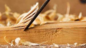
Woodcraft Ideas For Kids And Beginning Woodcrafters
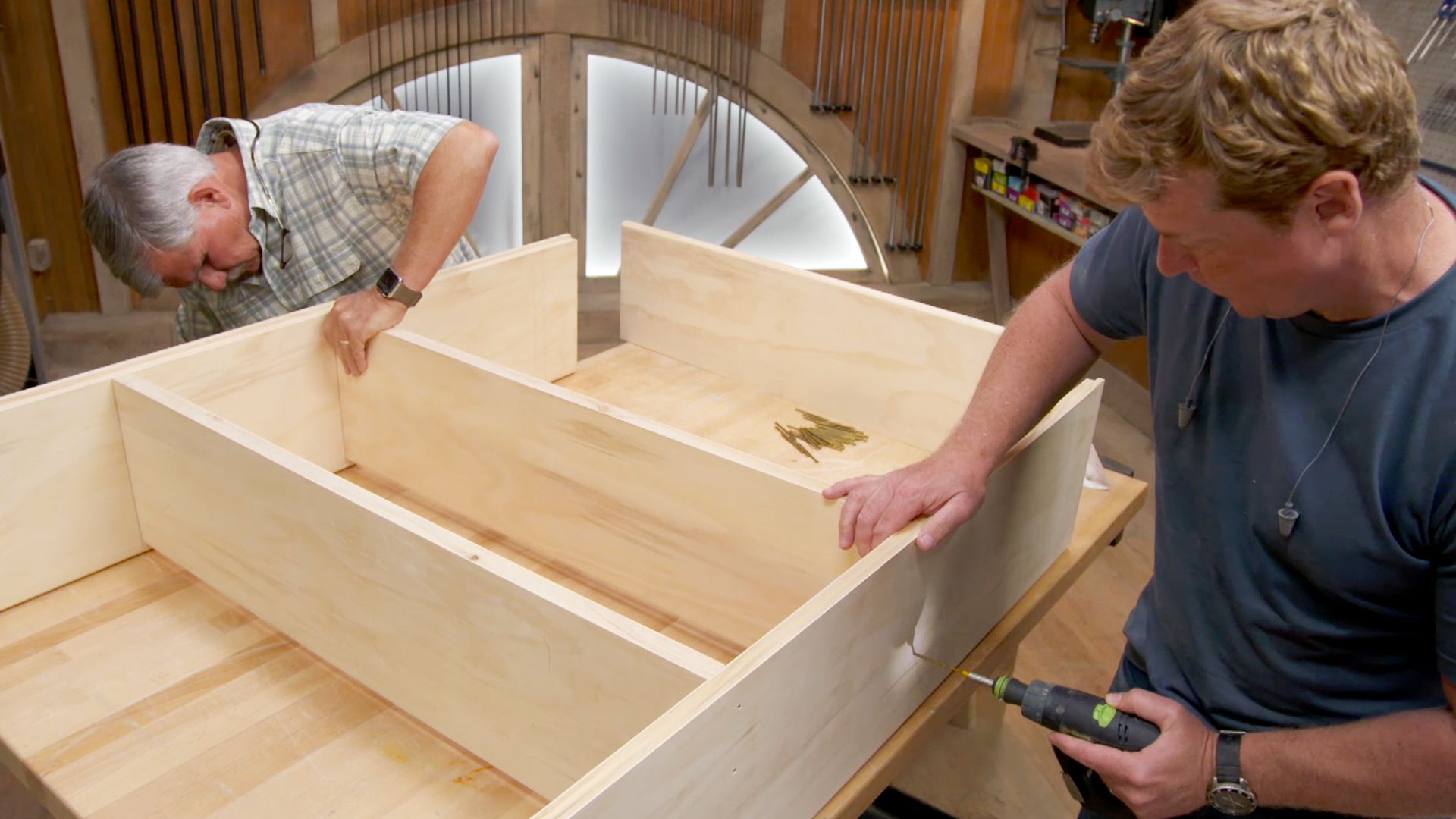
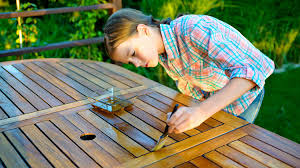
Woodcrafting can be one of the most enjoyable hobbies you'll find around. Not only is it enjoyable, but it's very productive, also. There are all kinds of woodcraft ideas you…
Read Full RecipeWoodcrafting can be one of the most enjoyable hobbies you'll find around. Not only is it enjoyable, but it's very productive, also. There are all kinds of woodcraft ideas you…
Read Full RecipeWoodcraft construction kits have been around for a good number of years now, but just recently started to really take off. We now find that there are a lot of…
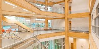
Read Full RecipeWell-made woodcraft furniture produced by skilled woodworkers has always been in demand, and that demand has grown with the realization that woodcraft furniture increased in value over time. Finely-made woodcraft…
Read Full RecipeAlmost anyone who has had success in any field of life will tell you that one of the secrets to living effectively is to have a plan. By having a…
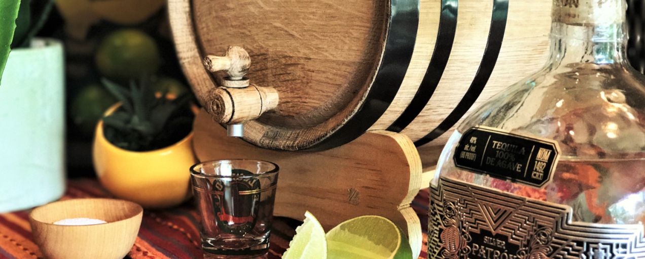
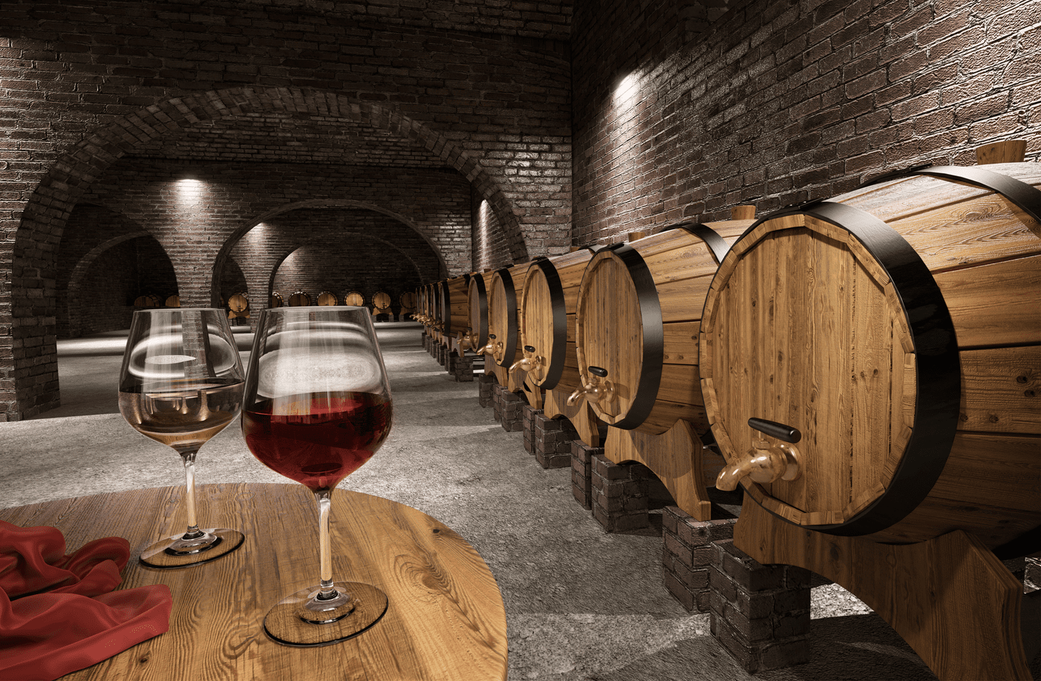
Read Full RecipeThe ancient art of coopering, often manifested in the form of barrel making, goes back thousands of years. Barrels were used by the Romans and the Gauls to store and…
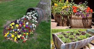
Read Full RecipeDo you have any old oak barrels sitting around and taking up space that could be put to better use? Well, if you do any sort of gardening you should…
Read Full RecipeA barrel is central on the storing and maturing processes of wine which are meant to provide a characteristic desirable flavor for the wine. This especially applies to additional costly…
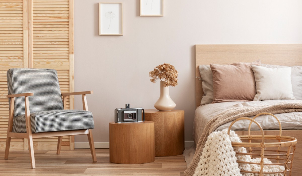
Read Full RecipeIf you're looking for new furniture for your home, then you're probably considering wooden furniture, such as dining sets, beds and wardrobes. If you're not convinced that wooden furniture is…
Read Full Recipe